TileDB Global Database for ICESat-2 ATL08 Data#

Important

If you use the database for your publications, please acknowledge that the dataset has been processed using icesat2DB:

Dombrowski, F., Besnard, S., Urbazaev, M., & Holcomb, A. icesat2DB [Computer software]. simonbesnard1/icesat2db.

Overview#

The publicly available TileDB global database, managed by the Global Land Monitoring group at GFZ-Potsdam, stores all processed ICESat-2 ATL08 version 7 data with a robust and scalable architecture. All granules for the ATL08 land and vegetation product have been ingested into the database, covering the full mission period from October 2018 onwards for all six ICESat-2 beams globally. The data is stored in a Ceph object storage managed by the GFZ data center. It enables efficient spatial, temporal, and attribute-based queries. This page provides an overview of the database setup, configuration, and access methods using the icesat2DB package.

Ceph Object Storage Configuration#

The TileDB global database utilises a Ceph object storage backend to efficiently manage and distribute ICESat-2 ATL08 data. Below are the key characteristics of the Ceph bucket:

Bucket Name: dog-ext.icesat2db.icesat2-atl08-v007
Access Endpoint: https://s3.gfz-potsdam.de
Region: eu-central-1
Access Control: Public
Query Support: Optimized for spatial and temporal queries

For users accessing the database programmatically, interactions with the Ceph bucket are abstracted by the icesat2DB package, which retrieves data seamlessly from TileDB. Advanced users with direct access to the Ceph storage layer may utilise S3-compatible tools (such as aws s3api or rclone) to interact with the data.

TileDB Database Configuration#

The database configuration defines key parameters for data storage, spatial tiling, and query efficiency. Data are written in 30×30-degree spatial tiles (latitude_tile: 6, longitude_tile: 6), producing approximately 60 occupied fragments globally. Annual temporal batching is used at ingest time so that one flush per year per tile is performed, minimising S3 open/close overhead while keeping memory usage bounded via the flush_every parameter.

Below is the structure of the configuration file used to build the TileDB database:

# database parameters
tiledb:
  storage_type: 's3'
  s3_bucket: "dog-ext.icesat2db.icesat2-atl08-v007"
  url: "https://s3.gfz-potsdam.de"
  overwrite: false
  temporal_batching: "annual"
  latitude_tile: 6
  longitude_tile: 6
  flush_every: 20000
  time_range:
    start_time: "2018-01-01"
    end_time: "2030-12-31"
  spatial_range:
    lat_min: -90.0
    lat_max: 90.0
    lon_min: -180.0
    lon_max: 180.0
  dimensions: ['latitude', 'longitude', 'time']
  s3_settings:
    connect_timeout_ms: "300000"
    request_timeout_ms: "600000"
    connect_max_tries: "10"
    multipart_part_size: "52428800"
    backoff_scale: "2.0"
    backoff_max_ms: "120000"
  cell_order: "hilbert"
  capacity: 100000
  use_filters: true
  spatial_zstd_level: 1
  timestamp_zstd_level: 2

The configuration file contains:

Storage Type: Specifies s3 for cloud-based Ceph storage.
Temporal Batching: annual — granules are batched by year before writing, reducing S3 open/close overhead.
Spatial Tiling: latitude_tile: 6 and longitude_tile: 6 define 30×30-degree write tiles, producing spatially localised TileDB fragments for efficient regional queries.
flush_every: Triggers a mid-batch write after every N granules to bound peak memory usage during ingest.
Time Range: Defines the global temporal coverage (mission start to end).
Spatial Range: Sets the global bounding box (full ±90° latitude, ±180° longitude).
Cell Order: Hilbert space-filling curve ordering for optimised spatial locality within fragments.
Compression: use_filters: true applies ByteShuffle+Zstd for float attributes and DoubleDelta+Zstd for time dimensions.

Note

The current database architecture writes one TileDB fragment per spatial tile per annual batch. Consolidation is not applied post-ingest; the spatial fragment structure is established at write time. Users are encouraged to provide feedback and suggestions for optimising the TileDB database configuration.

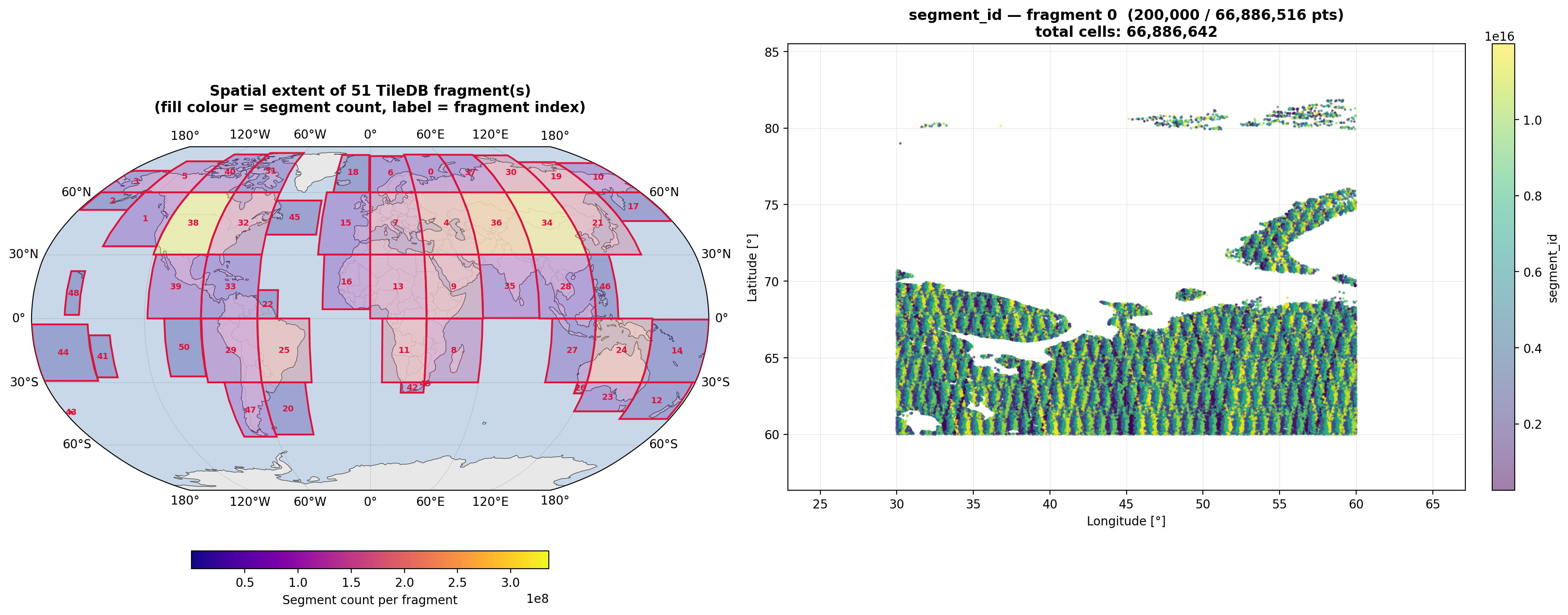
Data structure of the TileDB array — **Figure 1**: The data structure in the TileDB Global Database for ICESat-2 ATL08 Data.#

List of the available variables#

The database includes a wide range of variables from the ATL08 land and vegetation product, covering terrain elevation, canopy height metrics, quality flags, and ancillary data. Profile variables (e.g., canopy_h_metrics) store multi-element arrays per 100 m segment, expanded into indexed columns in the database. Sub-segment variables (e.g., h_canopy_20m) store values at 20 m resolution within each 100 m segment (5 values per segment).

Note

Profile variables canopy_h_metrics and canopy_h_metrics_abs contain 18 values per segment, each corresponding to a fixed percentile of the canopy height distribution. When queried, these are exposed as a named percentile coordinate:

ds.canopy_h_metrics.sel(percentile=50)   # median canopy height
ds.canopy_h_metrics.sel(percentile=95)   # 95th-percentile canopy height

The 18 percentile values are: 10, 15, 20, 25, 30, 35, 40, 45, 50, 55, 60, 65, 70, 75, 80, 85, 90, 95.

To fetch only a single percentile at query time (saving bandwidth by reading one column instead of all 18), use the variable:label syntax when calling get_data:

# Returns only the 50th-percentile column, renamed to 'canopy_h_metrics_p50'
ds = provider.get_data(variables=["canopy_h_metrics:50"], ...)
df = provider.get_data(variables=["canopy_h_metrics:50"], return_type="dataframe", ...)

Sub-segment variables h_canopy_20m, h_te_best_fit_20m, latitude_20m, longitude_20m, subset_can_flag, and subset_te_flag contain 5 values per segment, one per 20 m sub-segment. These are exposed as a named along_track_offset_m coordinate representing the midpoint of each 20 m bin within the 100 m segment:

ds.h_canopy_20m.sel(along_track_offset_m=50)   # centre 20 m bin of the 100 m segment
ds.h_canopy_20m.sel(along_track_offset_m=10)   # first 20 m bin

The 5 along-track offsets are: 10, 30, 50, 70, 90 metres.

The same single-label syntax applies to sub-segment variables:

# Returns only the centre 20 m bin, renamed to 'h_canopy_20m_50m'
ds = provider.get_data(variables=["h_canopy_20m:50"], ...)

Variable Descriptions#
Variable Name	Description	Units	Category
asr	Apparent surface reflectance	adimensional	Land Segment
atlas_pa	Off nadir pointing angle of the satellite	radians	Land Segment
beam_azimuth	Azimuth of the unit pointing vector for the reference photon in the local ENU frame	radians	Land Segment
beam_coelev	Co-elevation (direction from vertical) of the laser beam	radians	Land Segment
beam_id	Beam identifier (gt1l, gt2l, gt3l, gt1r, gt2r, gt3r)	adimensional	Reference
brightness_flag	Flag indicating a bright ground surface (e.g. snow-covered)	adimensional	Land Segment
can_noise	Number of noise photons falling within the canopy height per 100 m segment	count/meter	Canopy
can_quality_score	Canopy quality score based on coincident conditions	adimensional	Canopy
canopy_h_metrics	Canopy height metrics at 10-95th percentiles of the canopy relative height distribution (18 values per segment)	meters	Canopy
canopy_h_metrics_abs	Absolute canopy height metrics above WGS84 Ellipsoid at 10-95th percentiles (18 values per segment)	meters	Canopy
canopy_openness	Standard deviation of canopy photon heights, providing inference of canopy openness	adimensional	Canopy
canopy_rh_conf	Canopy relative height confidence flag (0=<5% canopy; 1=>5% canopy, <5% ground; 2=>5% canopy and ground)	adimensional	Canopy
centroid_height	Optical centroid height of canopy and ground photons above the reference ellipsoid	meters	Canopy
cloud_flag_atm	Cloud/aerosol confidence flag from ATL09 (0-10; >0 means aerosols or clouds may be present)	adimensional	Land Segment
cloud_fold_flag	Flag indicating likely cloud signal folded down from above 15 km	adimensional	Land Segment
delta_time	Mean GPS seconds since the ATLAS SDP epoch for the segment	seconds since 2018-01-01	Land Segment
delta_time_beg	GPS seconds since ATLAS SDP epoch for the first photon in the segment	seconds since 2018-01-01	Land Segment
delta_time_end	GPS seconds since ATLAS SDP epoch for the last photon in the segment	seconds since 2018-01-01	Land Segment
dem_flag	Source of the DEM height (0=None, 1=Arctic, 2=Global, 3=MSS, 4=Antarctic)	adimensional	Land Segment
dem_h	Best available DEM height above the WGS84 Ellipsoid at the geolocation point	meters	Land Segment
dem_removal_flag	Flag indicating >20% of segment removed due to failing DEM quality tests	adimensional	Land Segment
h_canopy	98th percentile of relative canopy heights within the segment above the estimated terrain surface	meters	Canopy
h_canopy_20m	Canopy height for each 20 m geosegment within the 100 m land segment (5 values per segment)	meters	Canopy
h_canopy_abs	98th percentile of absolute canopy heights above the WGS84 Ellipsoid	meters	Canopy
h_canopy_quad	Quadratic mean height of relative canopy photon heights above terrain	meters	Canopy
h_canopy_uncertainty	Uncertainty of the relative canopy height for the segment	meters	Canopy
h_dif_canopy	Difference between h_canopy and h_median_canopy	meters	Canopy
h_dif_ref	Difference between h_te_median and the reference DEM	meters	Land Segment
h_max_canopy	Maximum relative canopy height within segment (equivalent to RH100)	meters	Canopy
h_max_canopy_abs	Maximum absolute canopy height above WGS84 Ellipsoid within segment	meters	Canopy
h_mean_canopy	Mean relative canopy height within segment	meters	Canopy
h_mean_canopy_abs	Mean absolute canopy height above WGS84 Ellipsoid within segment	meters	Canopy
h_median_canopy	Median relative canopy height within segment (equivalent to RH50)	meters	Canopy
h_median_canopy_abs	Median absolute canopy height above WGS84 Ellipsoid within segment	meters	Canopy
h_min_canopy	Minimum relative canopy height within segment	meters	Canopy
h_min_canopy_abs	Minimum absolute canopy height above WGS84 Ellipsoid within segment	meters	Canopy
h_te_best_fit	Best-fit terrain elevation at the mid-point of each 100 m segment	meters	Terrain
h_te_best_fit_20m	Best-fit terrain height at the centre of each 20 m geosegment (5 values per segment)	meters	Terrain
h_te_interp	Interpolated terrain surface height above WGS84 Ellipsoid at segment midpoint	meters	Terrain
h_te_max	Maximum terrain photon height above WGS84 Ellipsoid within segment	meters	Terrain
h_te_mean	Mean terrain photon height above WGS84 Ellipsoid within segment	meters	Terrain
h_te_median	Median terrain photon height above WGS84 Ellipsoid within segment	meters	Terrain
h_te_min	Minimum terrain photon height above WGS84 Ellipsoid within segment	meters	Terrain
h_te_mode	Mode of terrain photon heights above WGS84 Ellipsoid within segment	meters	Terrain
h_te_rh25	Terrain elevation at the 25th percentile of classified ground photon heights	meters	Terrain
h_te_skew	Skewness of terrain photon heights above WGS84 Ellipsoid within segment	meters	Terrain
h_te_std	Standard deviation of terrain photon heights above WGS84 Ellipsoid (terrain roughness)	meters	Terrain
h_te_uncertainty	Uncertainty of the mean terrain height for the segment	meters	Terrain
last_seg_extend	Distance the last ATL08 segment is extended or overlapped with the previous segment	kilometers	Land Segment
latitude_20m	Centre latitude of 20 m geosegments within each 100 m land segment (5 values per segment)	degrees	Land Segment
layer_flag	Consolidated cloud/blowing snow flag (0=absent, 1=likely present)	adimensional	Land Segment
longitude_20m	Centre longitude of 20 m geosegments within each 100 m land segment (5 values per segment)	degrees	Land Segment
msw_flag	Multiple scattering warning flag (-1 to 5; 0=no scattering, 5=highest scattering)	adimensional	Land Segment
n_ca_photons	Number of photons classified as canopy within the segment	adimensional	Canopy
n_seg_ph	Total number of photons within each land segment	adimensional	Land Segment
n_te_photons	Number of photons classified as terrain within the segment	adimensional	Terrain
n_toc_photons	Number of photons classified as top of canopy within the segment	adimensional	Canopy
night_flag	Day/night flag derived from solar elevation (0=day, 1=night)	adimensional	Land Segment
ph_ndx_beg	Index (1-based) of the first photon in this land segment within the photon-rate data	adimensional	Land Segment
ph_removal_flag	Flag indicating >50% of segment photons removed due to failing quality tests	adimensional	Land Segment
photon_rate_can	Photon rate of canopy photons within each 100 m segment	s^-1	Canopy
photon_rate_can_nr	Noise-removed photon canopy rate within each 100 m segment	s^-1	Canopy
photon_rate_te	Photon rate of terrain photons within each 100 m segment	s^-1	Terrain
psf_flag	Flag set to 1 if the point spread function (sigma_atlas_land) exceeds 1 m	adimensional	Land Segment
rgt	Reference ground track number (1-1387)	adimensional	Land Segment
sat_flag	Saturation flag derived from full_sat_fract on ATL03, averaged over 5 geosegments	adimensional	Land Segment
sc_orient	Spacecraft orientation between forward, backward and transitional flight modes (0=backward, 1=forward, 2=transition)	adimensional	Orbit Information
segment_cover	Average Copernicus fractional canopy cover percentage for each 100 m segment	adimensional	Canopy
segment_id	Unique segment identifier	adimensional	Reference
segment_id_beg	Geolocation segment number of the first photon in the land segment	adimensional	Land Segment
segment_id_end	Geolocation segment number of the last photon in the land segment	adimensional	Land Segment
segment_landcover	UN-FAO land cover surface type from Copernicus Land Cover (ANC18) at 100 m	adimensional	Land Segment
segment_snowcover	Daily snow/ice cover flag (0=ice-free water, 1=snow-free land, 2=snow, 3=ice)	adimensional	Land Segment
segment_watermask	Water mask from the Global Raster Water Mask (ANC33) at 250 m resolution	adimensional	Land Segment
sigma_across	Total cross-track geolocation uncertainty due to PPD and POD knowledge	meters	Land Segment
sigma_along	Total along-track geolocation uncertainty due to PPD and POD knowledge	meters	Land Segment
sigma_atlas_land	Total vertical geolocation error due to ranging and local surface slope	meters	Land Segment
sigma_h	1-sigma uncertainty of the reference photon bounce point ellipsoid height	meters	Land Segment
sigma_topo	Total uncertainty including sigma_h plus geolocation uncertainty due to local slope	meters	Land Segment
snr	Signal-to-noise ratio of geolocated photons	adimensional	Land Segment
solar_azimuth	Direction (eastwards from north) of the sun vector at the laser ground spot	degrees_east	Land Segment
solar_elevation	Solar angle above or below the ellipsoid tangent plane at the laser spot	degrees	Land Segment
subset_can_flag	Quality flag for canopy segments derived from <100 m or <5 ATL03 20 m segments (5 values per segment)	adimensional	Canopy
subset_te_flag	Quality flag for terrain segments derived from <100 m or <5 ATL03 20 m segments (5 values per segment)	adimensional	Terrain
surf_type	Surface type flags (land, ocean, sea ice, land ice, inland water; 5 values per segment)	adimensional	Land Segment
te_quality_score	Terrain quality score based on coincident conditions	adimensional	Terrain
terrain_flg	Terrain flag indicating deviation above threshold from the reference DEM height	adimensional	Terrain
terrain_slope	Along-track slope of terrain computed by linear fit of terrain photons	meters	Terrain
toc_roughness	Standard deviation of top-of-canopy photon heights within segment	meters	Canopy
urban_flag	Flag indicating the segment is likely located over an urban area	adimensional	Land Segment

Accessing the database#

The icesat2DB Python package simplifies access to the TileDB global database. Below is an example workflow for querying data.

Example Code:

import geopandas as gpd
import icesat2db as isdb

# Instantiate the IceSat2Provider
provider = isdb.IceSat2Provider(
    storage_type='s3',
    s3_bucket="dog-ext.icesat2db.icesat2-atl08-v007",
    url="https://s3.gfz-potsdam.de"
)

# Load region of interest (ROI)
region_of_interest = gpd.read_file('path/to/region.geojson')

# Query data
atl08_data = provider.get_data(
    variables=["h_canopy", "h_te_best_fit"],
    query_type="bounding_box",
    geometry=region_of_interest,
    start_time="2019-01-01",
    end_time="2023-12-31",
    return_type='xarray'
)

Explanation:

IceSat2Provider: Initialises the provider with S3 storage details.
Region of Interest: Defines the geographic area for the query using a GeoJSON file.
Variables: Specifies the variables to extract (e.g., h_canopy, h_te_best_fit).
return_type: 'xarray' returns an xr.Dataset with coordinates and metadata attached; 'dataframe' returns a pd.DataFrame.

Examples and use cases#

Here are some example use cases:

Retrieve canopy height for a region:

atl08_data = provider.get_data(
    variables=["h_canopy", "h_max_canopy", "h_te_best_fit"],
    query_type="bounding_box",
    geometry=region_of_interest,
    start_time="2019-01-01",
    end_time="2023-12-31",
    return_type='xarray')

Apply quality filters when querying:

atl08_data = provider.get_data(
    variables=["h_canopy", "h_te_best_fit"],
    query_type="bounding_box",
    geometry=region_of_interest,
    start_time="2019-01-01",
    end_time="2023-12-31",
    return_type='xarray',
    night_flag="== 1",
    layer_flag="== 0")

Retrieve nearest shots to a point:

atl08_data = provider.get_data(
    variables=["h_canopy", "h_te_best_fit", "snr"],
    query_type="nearest",
    point=(13.4, 52.5),   # (longitude, latitude)
    num_shots=50,
    radius=0.5,
    start_time="2020-01-01",
    end_time="2023-12-31",
    return_type='dataframe')

Application: Global Canopy Height Dynamics#

This example demonstrates how to use the TileDB global database to analyse multi-temporal canopy height changes across the globe. The workflow queries h_canopy for two consecutive periods (2018-2021 and 2022-2025), aggregates the segments onto a custom equal-area hexagonal grid (~100 km diameter per cell), and maps the per-cell change in median canopy height.

The key steps are:

Query h_canopy for each period over the global bounding box (60°S-80°N) using IceSat2Provider.
Filter shots to the physically plausible canopy height range (2-60 m).
Aggregate shots to hex cells (minimum 100 shots per cell) and compute the median per cell.
Compute the per-cell difference Δh_canopy = period 2 − period 1 for hexes present in both periods.
Plot the baseline canopy height and the change map side-by-side in Equal Earth projection with fixed axis limits.

import geopandas as gpd
import pandas as pd
import matplotlib.pyplot as plt
import matplotlib as mpl
import numpy as np
from scipy.spatial import cKDTree
from pyproj import Transformer
from shapely.geometry import Polygon, box
import icesat2db as idb

# ── Style ──────────────────────────────────────────────────────────────────────
mpl.rcParams.update({
    'font.family': 'serif',
    'font.size': 16,
    'axes.titlesize': 13,
    'axes.labelsize': 12,
    'axes.linewidth': 0.5,
    'xtick.labelsize': 11,
    'ytick.labelsize': 11,
    'xtick.major.width': 0.3,
    'ytick.major.width': 0.3,
    'legend.fontsize': 12,
    'text.usetex': True,
})

# ── Config ─────────────────────────────────────────────────────────────────────
PROJ         = "+proj=eqearth +lon_0=0 +datum=WGS84 +units=m +no_defs"  # Equal Earth, seam at 30°W (Atlantic)
HEX_DIAMETER = 100_000        # metres (~100 km)
MIN_SHOTS    = 100
OUTPATH      = 'global_canopy_dynamics.png'

# Quality filters — applied server-side via TileDB before any data is transferred
# segment_landcover: Copernicus closed forest (111–116) + open forest (121–126)
_FOREST_CLASSES = [111, 112, 113, 114, 115, 116, 121, 122, 123, 124, 125, 126]
QUALITY_FILTERS = {
    "segment_landcover": f"in {_FOREST_CLASSES}",
    "h_canopy":          ">= 5 and <= 60",    # metres
    "n_ca_photons":      ">= 2 and <= 140",  # upper bound excludes noise misclassified as canopy
    "n_te_photons":      ">= 10",
}

GLOBAL_BBOX = gpd.GeoDataFrame(geometry=[box(-179.9, -60, 179.9, 80)], crs="EPSG:4326")
PERIODS = [
    ("2018-10-01", "2021-12-31"),
    ("2022-01-01", "2025-12-31"),
]

# ── Provider ───────────────────────────────────────────────────────────────────
provider = idb.IceSat2Provider(
    storage_type='s3',
    s3_bucket="dog-ext.icesat2db.icesat2-atl08-v007",
    url="https://s3.gfz-potsdam.de"
)

# ── Hex centers: vectorised, land-clipped, no polygons yet ────────────────────
def _proj_extent(lat_min=-60, lat_max=80):
    """
    Return (xmin, ymin, xmax, ymax) of the Equal Earth projection in metres.
    Robust to any lon_0: samples lons densely so both sides of the seam are hit.
    """
    _tr = Transformer.from_crs("EPSG:4326", PROJ, always_xy=True)
    sample_xs, _ = _tr.transform(np.linspace(-179.9, 179.9, 720), np.zeros(720))
    _, ymin = _tr.transform(0, lat_min)
    _, ymax = _tr.transform(0, lat_max)
    return sample_xs.min(), ymin, sample_xs.max(), ymax


def build_hex_centers(hex_diameter=HEX_DIAMETER):
    """
    Return (centers, hex_ids) where:
    centers  — (N, 2) float64 array of hex centres in PROJ
    hex_ids  — (N,)   int64  array of stable hex labels (original grid index)
    Ocean hexes carry no shots and are dropped automatically by MIN_SHOTS.
    """
    xmin, ymin, xmax, ymax = _proj_extent()

    r  = hex_diameter / 2
    dx = 3 / 2 * r
    dy = np.sqrt(3) * r

    cols = int((xmax - xmin) / dx) + 2
    rows = int((ymax - ymin) / dy) + 2

    # Vectorised centre computation — no Python loop
    col_idx = np.arange(cols)
    row_idx = np.arange(rows)
    col_flat, row_flat = np.meshgrid(col_idx, row_idx)
    col_flat = col_flat.ravel()
    row_flat = row_flat.ravel()

    cx = xmin + col_flat * dx
    cy = ymin + row_flat * dy + np.where(col_flat % 2 == 1, dy / 2, 0.0)

    centers = np.column_stack([cx, cy])
    hex_ids = np.arange(len(centers))
    return centers, hex_ids


print("Building hex centres...")
centers, hex_ids = build_hex_centers()
print(f"  {len(centers):,} hexes")

# Build KDTree and Transformer once — reused for both periods
tree    = cKDTree(centers)
to_proj = Transformer.from_crs("EPSG:4326", PROJ, always_xy=True)


# ── Fetch → filter → KDTree assign → aggregate ────────────────────────────────
def fetch_and_aggregate(provider, start, end):
    """
    Query one period, assign each shot to its nearest hex centre via KDTree
    (equivalent to polygon containment for a regular grid), then aggregate.
    No GeoDataFrame or shapely Point objects are created for the shots.
    """
    print(f"  Fetching {start} → {end}...")
    ds = provider.get_data(
        variables=["h_canopy"],
        query_type="bounding_box",
        geometry=GLOBAL_BBOX,
        start_time=start,
        end_time=end,
        return_type="dataframe",
        **QUALITY_FILTERS,
    )

    # Extract numpy arrays immediately — drop xarray and the DataFrame ASAP
    df = (
        ds[["h_canopy", "latitude", "longitude"]]
        .reset_index()[["latitude", "longitude", "h_canopy"]]
        .dropna(subset=["h_canopy"])
        .astype({"h_canopy": "float32", "latitude": "float32", "longitude": "float32"})
    )
    del ds
    print(f"  {len(df):,} shots after quality filter")

    lons      = df["longitude"].values
    lats      = df["latitude"].values
    h_canopy  = df["h_canopy"].values
    del df

    # Project to Equal Earth — pure numpy via pyproj, no GeoDataFrame
    px, py = to_proj.transform(lons, lats)
    del lons, lats

    # Nearest-centre assignment — parallel C code, no shapely objects
    # For a regular hex grid, nearest-centre == polygon containment (Voronoi identity)
    _, nn_idx = tree.query(np.column_stack([px, py]), workers=-1)
    del px, py
    assigned = hex_ids[nn_idx]
    del nn_idx

    agg = (
        pd.DataFrame({"hex_id": assigned, "h_canopy": h_canopy})
        .groupby("hex_id")["h_canopy"]
        .agg(h_canopy="median", n_shots="count")
    )
    del assigned, h_canopy

    return agg[agg["n_shots"] >= MIN_SHOTS][["h_canopy"]]


print("Processing period 1...")
agg1 = fetch_and_aggregate(provider, *PERIODS[0])
print(f"  {len(agg1):,} valid hexes")

print("Processing period 2...")
agg2 = fetch_and_aggregate(provider, *PERIODS[1])
print(f"  {len(agg2):,} valid hexes")

# ── Delta ──────────────────────────────────────────────────────────────────────
hex_df = (
    agg1.rename(columns={"h_canopy": "h_canopy_p1"})
        .join(agg2.rename(columns={"h_canopy": "h_canopy_p2"}), how="inner")
)
hex_df["delta_h_canopy"] = (hex_df["h_canopy_p2"] - hex_df["h_canopy_p1"]).astype("float32")
del agg1, agg2
print(f"  {len(hex_df):,} hexes with data in both periods")

# ── Polygons: created only for the hexes that survived all filters ─────────────
r       = HEX_DIAMETER / 2
angles  = np.linspace(0, 2 * np.pi, 7)[:-1]
offsets = np.stack([r * np.cos(angles), r * np.sin(angles)], axis=1)  # (6, 2)

pos_mask          = np.isin(hex_ids, hex_df.index.values)
surviving_centers = centers[pos_mask]
surviving_labels  = hex_ids[pos_mask]

# Broadcasting: (M, 1, 2) + (1, 6, 2) → (M, 6, 2)
vertices = surviving_centers[:, np.newaxis, :] + offsets[np.newaxis, :, :]
polys    = [Polygon(v) for v in vertices]

# Keep polygons in Equal Earth — converting to EPSG:4326 would break hexes
# that straddle the antimeridian (near ±180°), causing rendering artifacts
# over eastern Australia and the Pacific.
hex_gdf = gpd.GeoDataFrame(hex_df.reindex(surviving_labels), geometry=polys, crs=PROJ)
del hex_df, centers, hex_ids, vertices, polys

_xmin, _ymin, _xmax, _ymax = _proj_extent()

# ── Plot ───────────────────────────────────────────────────────────────────────
fig, axs = plt.subplots(2, 1, figsize=(16, 10), constrained_layout=True)
legend_kw = {"shrink": 0.45, "orientation": "vertical", "pad": 0.02}

hex_gdf.plot(
    column="h_canopy_p1", ax=axs[0],
    cmap="YlGnBu", edgecolor="none", legend=True,
    vmin=2, vmax=40,
    legend_kwds={**legend_kw, "label": r"Median $h_{\mathrm{canopy}}$ [m]"},
)
axs[0].set_xlim(_xmin, _xmax)
axs[0].set_ylim(_ymin, _ymax)
axs[0].set_title(r"Canopy Height Baseline --- 2018--2021", fontsize=14)
axs[0].set_xlabel("Easting (m, Equal Earth)")
axs[0].set_ylabel("Northing (m, Equal Earth)")
for sp in axs[0].spines.values(): sp.set_visible(False)

lim = np.percentile(hex_gdf["delta_h_canopy"].abs().dropna(), 95)
hex_gdf.plot(
    column="delta_h_canopy", ax=axs[1],
    cmap="BrBG", edgecolor="none", legend=True,
    vmin=-lim, vmax=lim,
    legend_kwds={**legend_kw, "label": r"$\Delta h_{\mathrm{canopy}}$ [m]"},
)
axs[1].set_xlim(_xmin, _xmax)
axs[1].set_ylim(_ymin, _ymax)
axs[1].set_title(r"$\Delta$ Canopy Height (2022--2025 vs.\ 2018--2021)", fontsize=14)
axs[1].set_xlabel("Easting (m, Equal Earth)")
axs[1].set_ylabel("Northing (m, Equal Earth)")
for sp in axs[1].spines.values(): sp.set_visible(False)

plt.savefig(OUTPATH, dpi=300, bbox_inches='tight')
plt.show()
print(f"Saved to {OUTPATH}")

The resulting figure shows (top) the median baseline canopy height for 2018-2021 and (bottom) the change in median canopy height between the two periods. Positive values (brown/green) indicate taller canopy in 2022-2025; negative values indicate a decline.

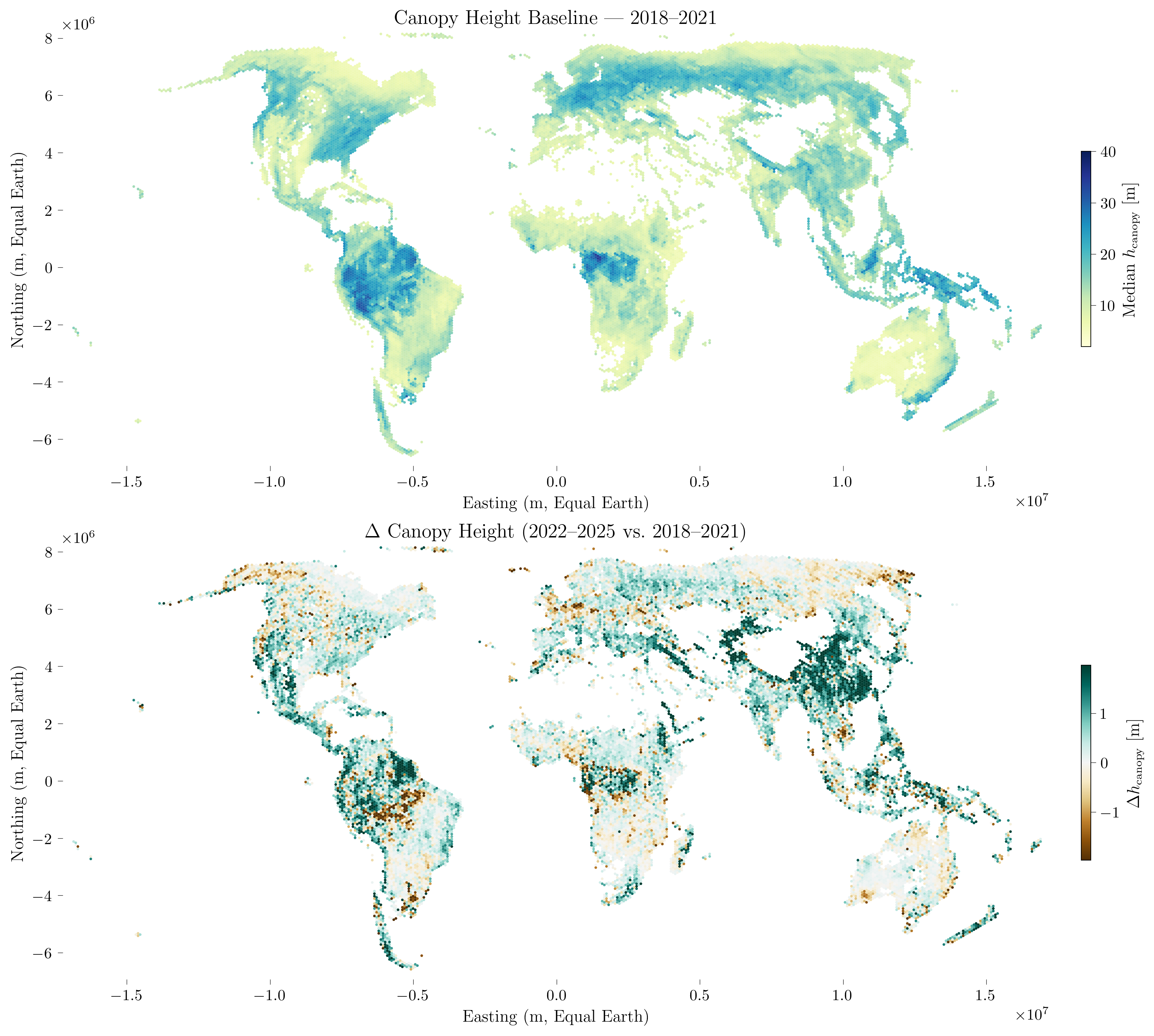
Global canopy height dynamics derived from ICESat-2 ATL08 — **Figure 2**: Global canopy height baseline (2018-2021, top) and change in median canopy height between 2022-2025 and 2018-2021 (bottom), aggregated on a custom equal-area hexagonal grid (~100 km diameter per cell, Equal Earth projection EPSG:8857). Only cells with at least 100 ATL08 segments in both periods are shown.#

Query Performance Benchmark#

The following script measures how query time scales with bounding box area by running 20 queries of increasing spatial extent centred on the same point, plus a full global archive query. Each query is repeated three times and the median wall-clock time is recorded.

import time
import geopandas as gpd
import matplotlib.pyplot as plt
import numpy as np
from shapely.geometry import box
import icesat2db as idb

CENTER_LON, CENTER_LAT = 10.0, 51.0
START_TIME, END_TIME   = "2020-01-01", "2020-12-31"
HALF_SIDES = np.linspace(0.25, 20.0, 20)   # degrees
N_REPEATS  = 3

provider = idb.IceSat2Provider(
    storage_type="s3",
    s3_bucket="dog-ext.icesat2db.icesat2-atl08-v007",
    url="https://s3.gfz-potsdam.de",
)

areas_km2, times_s, n_shots = [], [], []

for half in HALF_SIDES:
    geom = gpd.GeoDataFrame(
        geometry=[box(CENTER_LON - half, CENTER_LAT - half,
                      CENTER_LON + half, CENTER_LAT + half)],
        crs="EPSG:4326",
    )
    area_km2 = (2 * half) ** 2 * 111.0 * (111.0 * np.cos(np.radians(CENTER_LAT)))

    repeat_times, n = [], None
    for _ in range(N_REPEATS):
        t0 = time.perf_counter()
        result = provider.get_data(
            variables=["h_canopy"],
            query_type="bounding_box",
            geometry=geom,
            start_time=START_TIME,
            end_time=END_TIME,
            return_type="dataframe",
            use_polygon_filter=False,
        )
        repeat_times.append(time.perf_counter() - t0)
        if result is not None and n is None:
            n = len(result)

    areas_km2.append(area_km2)
    times_s.append(float(np.median(repeat_times)))
    n_shots.append(n or 0)

# Global archive query
GLOBAL_BBOX = gpd.GeoDataFrame(
    geometry=[box(-179.9, -60, 179.9, 80)], crs="EPSG:4326"
)
GLOBAL_AREA_KM2 = 150_000_000

global_times = []
for _ in range(N_REPEATS):
    t0 = time.perf_counter()
    provider.get_data(
        variables=["h_canopy"],
        query_type="bounding_box",
        geometry=GLOBAL_BBOX,
        start_time=START_TIME,
        end_time=END_TIME,
        return_type="dataframe",
        use_polygon_filter=False,
    )
    global_times.append(time.perf_counter() - t0)
GLOBAL_TIME_S = float(np.median(global_times))

# Plot
fig, ax = plt.subplots(figsize=(9, 5))
ax.scatter(areas_km2, times_s, color="steelblue", zorder=3)
ax.plot(areas_km2, times_s, color="steelblue", linewidth=1.2, alpha=0.6)

# Dashed break lines between regional and global points
x_break = (areas_km2[-1] * GLOBAL_AREA_KM2) ** 0.5
y_break = (times_s[-1]   * GLOBAL_TIME_S)   ** 0.5
ax.axvline(x_break, color="grey", linestyle=(0, (4, 4)), linewidth=0.8, alpha=0.7)
ax.axhline(y_break, color="grey", linestyle=(0, (4, 4)), linewidth=0.8, alpha=0.7)

# Global archive point
ax.scatter(GLOBAL_AREA_KM2, GLOBAL_TIME_S,
           color="tomato", marker="*", s=180, zorder=4)
ax.annotate("Global archive\n(~150 M km²)",
            xy=(GLOBAL_AREA_KM2, GLOBAL_TIME_S),
            xytext=(-90, 8), textcoords="offset points",
            fontsize=8, color="tomato",
            arrowprops=dict(arrowstyle="->", color="tomato", lw=0.8))

ax.set_xlabel("Bounding box area (km²)")
ax.set_ylabel("Query time (s)")
ax.set_xscale("log")
ax.set_yscale("log")
ax.set_yticks([1, 5, 10, 60, 300])
ax.set_yticklabels(["1 s", "5 s", "10 s", "1 min", "5 min"])
ax.grid(True, which="both", linestyle="--", linewidth=0.4, alpha=0.6)
plt.tight_layout()
plt.savefig("benchmark_query_scaling.png", dpi=150, bbox_inches="tight")

The figure below shows two complementary views of the benchmark results. Two regimes are visible in the absolute query time (left panel): for small extents (< ~3 M km²) time is nearly flat, dominated by S3 tile-open latency; above that threshold it scales roughly linearly with data volume. Regional queries up to ~12 M km² complete in under 5 seconds, and the full global archive (~150 M km²) returns in just over 1 minute.

The efficiency panel (right) confirms that larger queries are significantly cheaper per km²: the cost per unit area decreases by roughly three orders of magnitude from a small regional query to the full global archive, demonstrating that batching data access into large spatial extents is far more efficient than issuing many small queries.

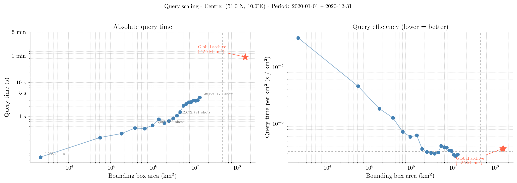
../_images/benchmark_query_scaling.png — **Figure**: icesat2DB query scaling for `h_canopy` over 2020, centred at 51°N 10°E. Left: absolute query time vs bounding box area. Right: query time normalised by area (s / km²) — lower is better. The red star marks the full global archive query (~67 s).#